Reproducing an example

The  beta distribution

Beta distribution function is “conjugate prior” for Bernoulli distribution (and others). It means that the “form” of posterior distribution is the same as the prior distribution.

The Bernoulli distribution:

p (y | θ) =

This “feature” of beta distribution allows us to keep using the same methods over and over because the posterior distribution’s form does not change. We can apply Bayesian steps in repetition.

There is a potential matter of confusion here:
Beta Distribution is different from the Beta function.

Following is the beta distribution:
p (θ | a, b) = beta(θ | a, b)
                     =

Where,

B(a, b) =

is a  normalizing constant or beta function.

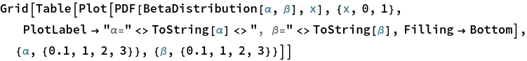
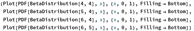
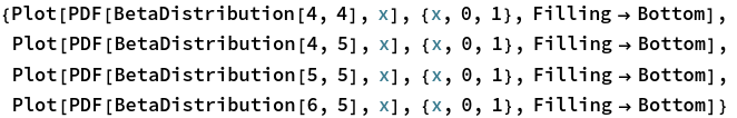
One of the most useful figures to understand what a beta distribution does, is Figure 6.1. It shows how the values of α and β change relative to each other. Let’s try to reproduce it.

Mathematica, of course, has the functions: BetaDistribution and Beta.

The image above has too much information. Let’s make it exactly like the Figure 6.1:

Exercises

Exercise 6.1

(A) Start with a prior distribution that expresses some uncertainty that a coin is fair: beta(θ|4,4). Flip the coin once; suppose we get a head. What is the posterior distribution?

(B) Use the posterior from the previous flip as the prior for the next flip. Suppose we flip again and get a head. Now what is the new posterior?

(C) Using that posterior as the prior for the next flip, flip a third time and get a tail. Now what is the new posterior?

(D) Do the same three updates, but in the order T, H, H instead  of H, H, T. Is the final posterior distribution the same for both orderings of the flip results?

Exploration

For (A) (B) and (C), we just have to increase α and β values as flip’s results come in. Plotting the results is simple, the same as shown in “Reproducing an example” section above.

Now for (D), the approach is exactly the same, the order of updating α and β changes:

Resulting distributions are the same, showing data order invariance.

Exercise 6.2

Suppose an election is approaching, and you are interested in knowing whether the general population prefers candidate A or candidate B. There is a just-published poll in the newspaper, which states that of 100 randomly sampled people, 58 preferred candidate A and the remainder preferred candidate B.

(A) Suppose that before the newspaper poll, your prior belief was a uniform distribution. What is the 95% HDI on your beliefs after learning of the newspaper poll results?

(B) You want to conduct a follow-up poll to narrow down your estimate of the population’s preference. In your follow-up poll, you randomly sample 100 other people and find that 57 prefer candidate A and the remainder prefer candidate B. Assuming peoples’ opinions have not changed between polls, what is the 95% HDI on the posterior?

Exploration

Since our prior beliefs about the matter is a uniform distribution, we don’t have to come up with our own values of α and β.
Let’ s plot the distribution of the original data to see what it looks like:

Let’s see where the peak lies, which tells us “Mode”:

To calculate 95% HDI, some finicky things are involved. They are finicky to me at least:

Thus, 95% HDI lies within the range of 0.482444 - 0.674524.

Next, we update our beliefs given new data we collect ourselves. The results of (A) will become our prior distribution.
We replicate the same process, but now with second set of samples included:

The mode has changed from 0.5816 to 0.5757.

Notice that the initial 95% HDI was {0.4824, 0.6745}, which changed to {0.5060, 0.6425} - it got narrower:

Exercises 6.3, 6.4, 6.5

These exercises are practically the same as 6.2. As results, they’re interesting. But implementation in Mathematica is just plugging in values of α and β and seeing the plots.
IOW, I am lazy.