ch_4 notebook-exclude

Initial Exploration

$RandomInteger [{0, 1}, 20]$

${1, 1, 1, 1, 0, 0, 1, 0, 0, 1, 0, 1, 1, 1, 0, 0, 0, 1, 0, 0}$

$RandomVariate [UniformDistribution [{0, 1}]]$

$0.6531459162175581$

$Count [RandomInteger [{0, 1}, 20], 0]$

$8$

$ListLinePlot [Table [Accumulate [RandomReal [{- 1, 1}, 250]], {3}], Filling \to Axis, PlotLegends \to {one, two, three}]$

$Accumulate [RandomInteger [{0, 1}, 10]]$

${1, 1, 2, 2, 3, 4, 5, 5, 6, 7}$

$ListLinePlot [%]$

$Table [RandomInteger [{0, 1}, 1], 10]$

$MovingAverage [{{0}, {1}, {1}, {1}, {0}, {1}, {0}, {1}, {0}, {1}}]$

$Accumulate [RandomInteger [BernoulliDistribution [0.5], 1000]] / Range [1000] // ListPlot$

$Accumulate [RandomVariate [NormalDistribution [], 5000]] / Range [5000] // ListPlot$

$ListPlot [RandomVariate [NormalDistribution [], 1000], Filling \to Axis]$

$ListPlot [RandomVariate [GeometricDistribution [1 / 2], 50], Filling \to Axis]$

$Accumulate [RandomInteger [{0, 1}, 100]] / Range [100] // ListPlot$

$Plot [6 x (1 - x), {x, 0, 1}, Filling -> Bottom]$

$Integrate [6 x (1 - x) x, {x, 0, 1}]$

$\frac{1}{2}$

$\int_{0}^{1} 6 x (1 - x) x ⅆ x$

$\frac{1}{2}$

$data = SemanticImport [/Users/codingquark/Documents/Wolfram Mathematica/doing_bayesian_data_analysis/DBDA2Eprograms/HairEyeColor.csv]$

$Mean [data]$

$ Hair \to \frac{1}{16} (4 Black + 4 Blond + 4 Brown + 4 Red), Eye \to \frac{1}{16} (4 Blue + 4 Brown + 4 Green + 4 Hazel), Count \to 37 $

$Length [data]$

$16$

$Normal [data]$

${ Hair \to Black, Eye \to Blue, Count \to 20 ,  Hair \to Black, Eye \to Brown, Count \to 68 ,  Hair \to Black, Eye \to Green, Count \to 5 ,  Hair \to Black, Eye \to Hazel, Count \to 15 ,  Hair \to Blond, Eye \to Blue, Count \to 94 ,  Hair \to Blond, Eye \to Brown, Count \to 7 ,  Hair \to Blond, Eye \to Green, Count \to 16 ,  Hair \to Blond, Eye \to Hazel, Count \to 10 ,  Hair \to Brown, Eye \to Blue, Count \to 84 ,  Hair \to Brown, Eye \to Brown, Count \to 119 ,  Hair \to Brown, Eye \to Green, Count \to 29 ,  Hair \to Brown, Eye \to Hazel, Count \to 54 ,  Hair \to Red, Eye \to Blue, Count \to 17 ,  Hair \to Red, Eye \to Brown, Count \to 26 ,  Hair \to Red, Eye \to Green, Count \to 14 ,  Hair \to Red, Eye \to Hazel, Count \to 14 }$

$data [Histogram, Count]$

$data [GroupBy [Hair], Total, Count]$

$data [GroupBy [Eye], Total, Count]$

$data [All, Count] // Total$

$592$

$data [GroupBy [Hair], Mean, Count]$

$data [GroupBy [Eye], Mean, Count]$

$data$

$titanic = ExampleData [{Dataset, Titanic}]$

$titanic [Histogram, age]$

$titanic [GroupBy [Key [sex]], Counts, class]$

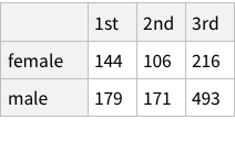
Watch https://www.wolfram.com/broadcast/video.php?c=377&p=2&v=1258

$data [Histogram, Count]$

$data [ListPlot, Count]$

$data [GroupBy [Hair], GroupBy [Eye]]$

$592$

$data [Mean, Count]$

$37$

$data [Median, Count]$

$\frac{37}{2}$

$data [Counts, Hair]$

$data [Counts, Eye]$

$data [MinMax, Count]$

$data [StandardDeviation, Count]$

$\sqrt{\frac{6314}{5}}$

$PieChart [data [GroupBy [Eye], Total, Count], ChartLegends -> Automatic]$

$PieChart [data [GroupBy [Hair], Total, Count], ChartLegends -> Automatic]$

$data [GroupBy [Eye]] // Normal$

$ Blue \to { Hair \to Black, Eye \to Blue, Count \to 20 ,  Hair \to Blond, Eye \to Blue, Count \to 94 ,  Hair \to Brown, Eye \to Blue, Count \to 84 ,  Hair \to Red, Eye \to Blue, Count \to 17 }, Brown \to { Hair \to Black, Eye \to Brown, Count \to 68 ,  Hair \to Blond, Eye \to Brown, Count \to 7 ,  Hair \to Brown, Eye \to Brown, Count \to 119 ,  Hair \to Red, Eye \to Brown, Count \to 26 }, Green \to { Hair \to Black, Eye \to Green, Count \to 5 ,  Hair \to Blond, Eye \to Green, Count \to 16 ,  Hair \to Brown, Eye \to Green, Count \to 29 ,  Hair \to Red, Eye \to Green, Count \to 14 }, Hazel \to { Hair \to Black, Eye \to Hazel, Count \to 15 ,  Hair \to Blond, Eye \to Hazel, Count \to 10 ,  Hair \to Brown, Eye \to Hazel, Count \to 54 ,  Hair \to Red, Eye \to Hazel, Count \to 14 } $

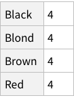
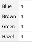
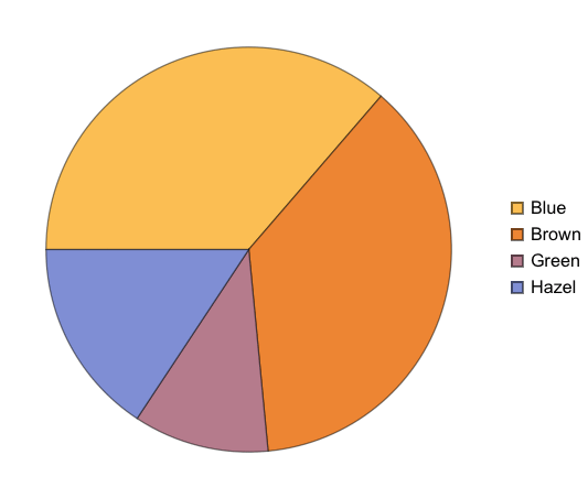
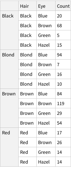
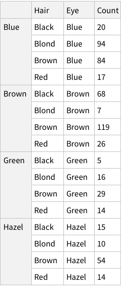
Given the structure so far, we need to figure out a way to have named rows, nested with further named rows. Like so: {“Brown Eye”->{“Black Hair”->4, “Blond Hair”->10}, “Blue Eye”->...}
Not sure if this should be done at import time, or as the next step after import.

Importing Data

How should it look like?

We want our Hair + Eye colour data to be structured “nicely” before we start doing analysis. What is this “nice” structure?

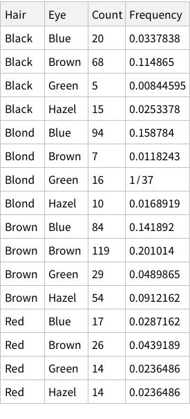
If imported simply, this is what it looks like:

This structure is not bad, it correctly figures out that the first row of the CSV is column names. But is this how we want things to be? Could we have more structure to it?

One approach can be to add some named rows. For example, we can imagine that the actual data point in the entire dataset is the `Count` column, rest are just names! Which means, we can have rows of rows.

Let’s try. What does the structure look like?

$planets = ExampleData [{Dataset, Planets}]$

$planets // Normal$

$ Mercury \to  Mass \to, Radius \to, Moons \to   , Venus \to  Mass \to, Radius \to, Moons \to   , Earth \to  Mass \to, Radius \to, Moons \to  Moon \to  Mass \to, Radius \to   , Mars \to  Mass \to, Radius \to, Moons \to  Phobos \to  Mass \to, Radius \to , Deimos \to  Mass \to, Radius \to   , Jupiter \to  Mass \to, Radius \to, Moons \to  Metis \to  Mass \to, Radius \to , Adrastea \to  Mass \to, Radius \to , Amalthea \to  Mass \to, Radius \to , Thebe \to  Mass \to, Radius \to , Io \to  Mass \to, Radius \to , Europa \to  Mass \to, Radius \to , Ganymede \to  Mass \to, Radius \to , Callisto \to  Mass \to, Radius \to , Themisto \to  Mass \to, Radius \to , Leda \to  Mass \to, Radius \to , Himalia \to  Mass \to, Radius \to , Lysithea \to  Mass \to, Radius \to , Elara \to  Mass \to, Radius \to , S/2000 J11 \to  Mass \to Missing [NotAvailable], Radius \to , S/2003 J12 \to  Mass \to Missing [NotAvailable], Radius \to , Carpo \to  Mass \to Missing [NotAvailable], Radius \to , Euporie \to  Mass \to, Radius \to , S/2003 J3 \to  Mass \to Missing [NotAvailable], Radius \to , S/2003 J18 \to  Mass \to Missing [NotAvailable], Radius \to , Orthosie \to  Mass \to, Radius \to , Euanthe \to  Mass \to, Radius \to , Harpalyke \to  Mass \to, Radius \to , Praxidike \to  Mass \to, Radius \to , Thyone \to  Mass \to, Radius \to , S/2003 J16 \to  Mass \to Missing [NotAvailable], Radius \to , Iocaste \to  Mass \to, Radius \to , Mneme \to  Mass \to Missing [NotAvailable], Radius \to , Hermippe \to  Mass \to, Radius \to , Thelxinoe \to  Mass \to Missing [NotAvailable], Radius \to , Helike \to  Mass \to Missing [NotAvailable], Radius \to , Ananke \to  Mass \to, Radius \to , S/2003 J15 \to  Mass \to Missing [NotAvailable], Radius \to , Eurydome \to  Mass \to, Radius \to , Arche \to  Mass \to Missing [NotAvailable], Radius \to , Herse \to  Mass \to Missing [NotAvailable], Radius \to , Pasithee \to  Mass \to, Radius \to , S/2003 J10 \to  Mass \to Missing [NotAvailable], Radius \to , Chaldene \to  Mass \to, Radius \to , Isonoe \to  Mass \to, Radius \to , Erinome \to  Mass \to, Radius \to , Kale \to  Mass \to, Radius \to , Aitne \to  Mass \to, Radius \to , Taygete \to  Mass \to, Radius \to , S/2003 J9 \to  Mass \to Missing [NotAvailable], Radius \to , Carme \to  Mass \to, Radius \to , Sponde \to  Mass \to, Radius \to , Megaclite \to  Mass \to, Radius \to , S/2003 J5 \to  Mass \to Missing [NotAvailable], Radius \to , S/2003 J19 \to  Mass \to Missing [NotAvailable], Radius \to , S/2003 J23 \to  Mass \to Missing [NotAvailable], Radius \to , Kalyke \to  Mass \to, Radius \to , Kore \to  Mass \to Missing [NotAvailable], Radius \to , Pasiphae \to  Mass \to, Radius \to , Eukelade \to  Mass \to Missing [NotAvailable], Radius \to , S/2003 J4 \to  Mass \to Missing [NotAvailable], Radius \to , Sinope \to  Mass \to, Radius \to , Hegemone \to  Mass \to Missing [NotAvailable], Radius \to , Aoede \to  Mass \to Missing [NotAvailable], Radius \to , Kallichore \to  Mass \to Missing [NotAvailable], Radius \to , Autonoe \to  Mass \to, Radius \to , Callirrhoe \to  Mass \to, Radius \to , Cyllene \to  Mass \to Missing [NotAvailable], Radius \to , S/2003 J2 \to  Mass \to Missing [NotAvailable], Radius \to   , Saturn \to  Mass \to, Radius \to, Moons \to  Tarqeq \to  Mass \to Missing [NotAvailable], Radius \to , Pan \to  Mass \to, Radius \to , Daphnis \to  Mass \to Missing [NotAvailable], Radius \to , Atlas \to  Mass \to, Radius \to , Prometheus \to  Mass \to, Radius \to , Pandora \to  Mass \to, Radius \to , Epimetheus \to  Mass \to, Radius \to , Janus \to  Mass \to, Radius \to , Aegaeon \to  Mass \to Missing [NotAvailable], Radius \to , Mimas \to  Mass \to, Radius \to , Methone \to  Mass \to Missing [NotAvailable], Radius \to , Anthe \to  Mass \to, Radius \to , Pallene \to  Mass \to Missing [NotAvailable], Radius \to , Enceladus \to  Mass \to, Radius \to , Tethys \to  Mass \to, Radius \to , Calypso \to  Mass \to, Radius \to , Telesto \to  Mass \to, Radius \to , Polydeuces \to  Mass \to Missing [NotAvailable], Radius \to , Dione \to  Mass \to, Radius \to , Helene \to  Mass \to, Radius \to , Rhea \to  Mass \to, Radius \to , Titan \to  Mass \to, Radius \to , Hyperion \to  Mass \to, Radius \to , Iapetus \to  Mass \to, Radius \to , Kiviuq \to  Mass \to, Radius \to , Ijiraq \to  Mass \to, Radius \to , Phoebe \to  Mass \to, Radius \to , Paaliaq \to  Mass \to, Radius \to , Skathi \to  Mass \to, Radius \to , Albiorix \to  Mass \to, Radius \to , S/2007 S2 \to  Mass \to, Radius \to , Bebhionn \to  Mass \to Missing [NotAvailable], Radius \to , Erriapo \to  Mass \to, Radius \to , Siarnaq \to  Mass \to, Radius \to , Skoll \to  Mass \to Missing [NotAvailable], Radius \to , Tarvos \to  Mass \to, Radius \to , Greip \to  Mass \to Missing [NotAvailable], Radius \to , S/2004 S13 \to  Mass \to Missing [NotAvailable], Radius \to , Hyrrokkin \to  Mass \to Missing [NotAvailable], Radius \to , Mundilfari \to  Mass \to, Radius \to , S/2006 S1 \to  Mass \to Missing [NotAvailable], Radius \to , Jarnsaxa \to  Mass \to Missing [NotAvailable], Radius \to , Narvi \to  Mass \to, Radius \to , Bergelmir \to  Mass \to Missing [NotAvailable], Radius \to , S/2004 S17 \to  Mass \to Missing [NotAvailable], Radius \to , Suttungr \to  Mass \to, Radius \to , Hati \to  Mass \to Missing [NotAvailable], Radius \to , S/2004 S12 \to  Mass \to Missing [NotAvailable], Radius \to , Bestla \to  Mass \to Missing [NotAvailable], Radius \to , Farbauti \to  Mass \to Missing [NotAvailable], Radius \to , Thrymr \to  Mass \to, Radius \to , S/2007 S3 \to  Mass \to Missing [NotAvailable], Radius \to , Aegir \to  Mass \to Missing [NotAvailable], Radius \to , S/2004 S7 \to  Mass \to Missing [NotAvailable], Radius \to , S/2006 S3 \to  Mass \to Missing [NotAvailable], Radius \to , Kari \to  Mass \to Missing [NotAvailable], Radius \to , Fenrir \to  Mass \to Missing [NotAvailable], Radius \to , Surtur \to  Mass \to Missing [NotAvailable], Radius \to , Ymir \to  Mass \to, Radius \to , Loge \to  Mass \to Missing [NotAvailable], Radius \to , Fornjot \to  Mass \to Missing [NotAvailable], Radius \to   , Uranus \to  Mass \to, Radius \to, Moons \to  Cordelia \to  Mass \to, Radius \to , Ophelia \to  Mass \to, Radius \to , Bianca \to  Mass \to, Radius \to , Cressida \to  Mass \to, Radius \to , Desdemona \to  Mass \to, Radius \to , Juliet \to  Mass \to, Radius \to , Portia \to  Mass \to, Radius \to , Rosalind \to  Mass \to, Radius \to , Cupid \to  Mass \to Missing [NotAvailable], Radius \to , Belinda \to  Mass \to, Radius \to , Perdita \to  Mass \to Missing [NotAvailable], Radius \to , Puck \to  Mass \to, Radius \to , Mab \to  Mass \to Missing [NotAvailable], Radius \to , Miranda \to  Mass \to, Radius \to , Ariel \to  Mass \to, Radius \to , Umbriel \to  Mass \to, Radius \to , Titania \to  Mass \to, Radius \to , Oberon \to  Mass \to, Radius \to , Francisco \to  Mass \to Missing [NotAvailable], Radius \to , Caliban \to  Mass \to, Radius \to , Stephano \to  Mass \to, Radius \to , Trinculo \to  Mass \to, Radius \to , Sycorax \to  Mass \to, Radius \to , Margaret \to  Mass \to Missing [NotAvailable], Radius \to , Prospero \to  Mass \to, Radius \to , Setebos \to  Mass \to, Radius \to , Ferdinand \to  Mass \to Missing [NotAvailable], Radius \to   , Neptune \to  Mass \to, Radius \to, Moons \to  Naiad \to  Mass \to, Radius \to , Thalassa \to  Mass \to, Radius \to , Despina \to  Mass \to, Radius \to , Galatea \to  Mass \to, Radius \to , Larissa \to  Mass \to, Radius \to , Proteus \to  Mass \to, Radius \to , Triton \to  Mass \to, Radius \to , Nereid \to  Mass \to, Radius \to , Halimede \to  Mass \to Missing [NotAvailable], Radius \to , Sao \to  Mass \to Missing [NotAvailable], Radius \to , Laomedeia \to  Mass \to Missing [NotAvailable], Radius \to , Psamathe \to  Mass \to Missing [NotAvailable], Radius \to , Neso \to  Mass \to Missing [NotAvailable], Radius \to    $

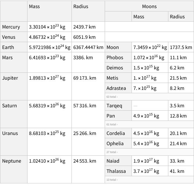
Okay, now that we know how data is represented, we can try manually creating a row or two for our data.

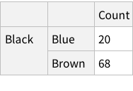
$dataset = Dataset [<| Black -> <| Blue -> <| Count -> 20 |>, <| Brown -> <| Count -> 68 |> |> |> |>]$

Does this look good? We don’t have column names for Hair and Eye, but we do for Count. Is that normal? If you look at the Moons in the planet dataset, you can see that the names of of moons are not column-named, but their properties are column-named. Which is analogous to what we have for our dataset as well.

Let’s finalise on this structure for now, and find out how to convert the imported data.

Structuring Imported Dataset

So far, I have not found any simple way to morph the dataset. The important note found so far is that we cannot modify existing Dataset, but instead have to create new Dataset with the structure we want. What this means, is that we will have to define Column/Row structure and select proper Count columns for the new Dataset definition.

This manual approach is too much hassle. And figuring out “script-like” way to change the structure is not attractive right now.

Hence, we will try to roll with what we have and see what happens when we try doing operations on the data.

References

https://www.wolfram.com/broadcast/video.php?c=377&p=2&v=1258

https://www.youtube.com/watch?v=XN8Y177doEE

https://www.wolfram.com/wolfram-u/courses/data-science/becoming-a-data-curator-dat906/

Basic Analysis

Exercises from 4.6

Exercise 4.1

The eye-color hair-color data is frequencies of eye and hair color for males and females. Run the (some, we are going to ignore them) R code.

In your write-up, include each line above and its results. Explain what each line does (in a bit more detail than the inline comments). Extend above commands by also computing the probabilities of the hair colors given brown eyes, and the probabilities of the eye colors given Brown hair.

First, let’s import the data and show it.

Run equivalent of:

Funnily enough, the R code given by the book loads the CSV, generates Male/Female split, and then store in the variable “HairEyeColor”. The “sum” application then gives the data we have got already!

Next line is dividing each cell by the total.

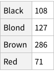
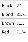
To find total counts of each hair-color:

$hairfrequencydataset = dataset [GroupBy [Hair], Total, Count]$

Like we added the Frequency column above for all rows, do the same but for the grouped data:

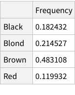
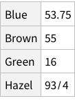
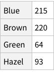
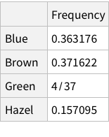
$hairproportions = hairfrequencydataset [All, <| Frequency -> #1 / counttotal |> &]$

Same operations now for eye colors:

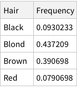
Calculate conditional probability of Hair, given Blue eye color (table 4.2):

$haireyeproportion [Select [#Eye == Blue &]] [All, <| Hair -> #Hair, Frequency -> N [#Frequency / eyeproportions [Blue, Frequency]] |> &]$

Calculate conditional probability of hair colors given brown eyes:

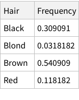
$haireyeproportion [Select [#Eye == Brown &]] [All, <| Hair -> #Hair, Frequency -> N [#Frequency / eyeproportions [Brown, Frequency]] |> &]$

Calculate conditional probability of eye colors given brown hair:

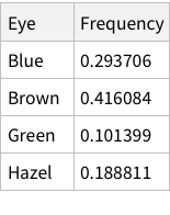
$haireyeproportion [Select [#Hair == Brown &]] [All, <| Eye -> #Eye, Frequency -> N [#Frequency / hairproportions [Brown, Frequency]] |> &]$

Let’s now try to understand, verbally, what the exercise was about.

We were given raw counts for hair+eye colour combos. Just like one of the section in the chapter, we wanted to get to finding out conditional probabilities.

To get to conditional probabilities, we needed some basic information derived first:

Proportions of each hair+eye colour combo

Proportions of each hair colour

Proportions of each eye colour

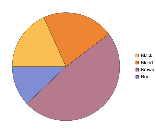
When we calculate hair+eye proportions, we are calculating joint probabilities. For example, the probability of finding someone with both Brown eyes and Black hair is 0.11 i.e. 11% and so on.

When we calculate the proportions of only hair or only eye colours, we are measuring probability of finding, for example, a person with black hair; a person with blue eyes and so on. For example, the probability of finding a person with Black hair is 0.18 / 18%; a person with Brown eyes is 0.37 / 37%

Finally, we can use the derived information to calculate conditional probabilities. To calculate the probability of a person having Hazel eyes, given we know that the person has Blond hair we need to divide independent probability by marginal probability. So, for the specific case, the calculation is: 0.0168919/0.214527 = 0.078 (~7%)

Thus ends a successful Exercise 4.1! Notice how the entire exercise was about calculating proportions in various ways and it did not feel the way it did when reading the section of the book.

Exercise 4.2

Modify the coin flipping program in Section 4.5 to simulate a biased coin that has p(H)=0.8. Change the height of the reference line in the plot to match p(H). Comment your code.

Okay, this is more involved since it is mainly about R code. We will have to first write code to simulate coin flips, then make the coin flips biased.

Alright, let’s think about this. The R code uses `sample` function that takes probability values with with to take the samples. We need something similar in Mathematica. But what is our real goal? We want to flip a coin - [H,T]. And when it is flipped we want to specify how biased the coin is. Having flipped the coin N times, we want to plot the running proportion of H and know the end proportion.

First, we have RandomVariate function that can take some distribution. The one we might find useful is DiscreteUniformDistribution. Let’s try.

$RandomVariate [DiscreteUniformDistribution [{0, 1}], 10] // Short$

${1, 0, 0, 0, 1, 1, 0, 0, 1, 1}$

$Histogram [RandomVariate [DiscreteUniformDistribution [{0, 1}], 500]]$

$tosses = RandomVariate [DiscreteUniformDistribution [{0, 1}], 500];$

$N [\frac{Count [tosses, 1]}{500}]$

$0.456$

$N [\frac{Count [tosses, 0]}{500}]$

$0.544$

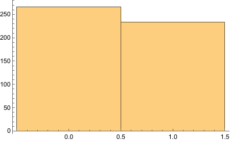
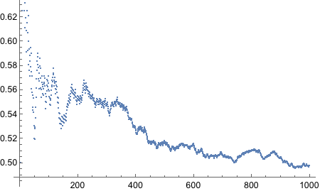
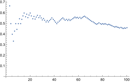
There, we got the end proportions of the fair die after 500 tosses.

$manytosses = RandomVariate [DiscreteUniformDistribution [{0, 1}], 50000];$

$ListPlot [Accumulate [\frac{manytosses}{Length [manytosses]}]]$

$ListLinePlot [Accumulate [Select [tosses, # == 1 &]]]$

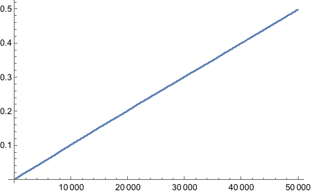
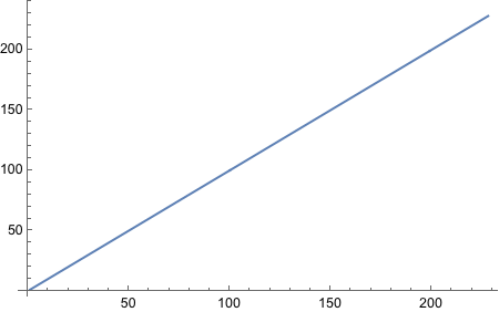
Still no idea how to get “running proportion”! FoldList works, but does not give access to current index of the list. MapIndex does not keep track of previous elements. Looks like we will have to write our own function. Not fun, I must say.

Stolen the following code from https://mathematica.stackexchange.com/questions/190503/how-to-make-foldlistindexed-ie-foldlist-with-an-index-or-iterator

${x, f [x, a, 1], f [f [x, a, 1], b, 2], f [f [f [x, a, 1], b, 2], c, 3], f [f [f [f [x, a, 1], b, 2], c, 3], d, 4]}$

$fewtosses = {1, 1, 0, 1, 1, 0, 1, 0, 0, 0}$

${1, 1, 0, 1, 1, 0, 1, 0, 0, 0}$

This approach may not be the thing we want. What we want is a list: ${\frac{1}{1}, \frac{2}{2}, \frac{2}{3}, \frac{3}{4}, \frac{4}{5}, \frac{4}{6}, \frac{5}{7}, \frac{5}{8}, \frac{5}{9}, \frac{5}{10}}$ and so on.

$For [i = 1; res = {}, i <= Length [tosses], i ++, AppendTo [res, Last @ \frac{FoldList [Plus, 0, tosses [[;; i]]]}{i}]]$

$ListLinePlot [res]$

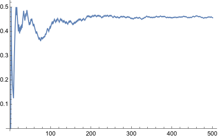
Well what do we have here! It worked! It is the ugliest way to do things because it is not functional, but it got the job done. We will refine this somehow.

$MapIndexed [\frac{FoldList [Plus, 0, fewtosses [[;; First [#2]]]]}{First [#2]} &, fewtosses]$

${{0, 1}, {0, \frac{1}{2}, 1}, {0, \frac{1}{3}, \frac{2}{3}, \frac{2}{3}}, {0, \frac{1}{4}, \frac{1}{2}, \frac{1}{2}, \frac{3}{4}}, {0, \frac{1}{5}, \frac{2}{5}, \frac{2}{5}, \frac{3}{5}, \frac{4}{5}}, {0, \frac{1}{6}, \frac{1}{3}, \frac{1}{3}, \frac{1}{2}, \frac{2}{3}, \frac{2}{3}}, {0, \frac{1}{7}, \frac{2}{7}, \frac{2}{7}, \frac{3}{7}, \frac{4}{7}, \frac{4}{7}, \frac{5}{7}}, {0, \frac{1}{8}, \frac{1}{4}, \frac{1}{4}, \frac{3}{8}, \frac{1}{2}, \frac{1}{2}, \frac{5}{8}, \frac{5}{8}}, {0, \frac{1}{9}, \frac{2}{9}, \frac{2}{9}, \frac{1}{3}, \frac{4}{9}, \frac{4}{9}, \frac{5}{9}, \frac{5}{9}, \frac{5}{9}}, {0, \frac{1}{10}, \frac{1}{5}, \frac{1}{5}, \frac{3}{10}, \frac{2}{5}, \frac{2}{5}, \frac{1}{2}, \frac{1}{2}, \frac{1}{2}, \frac{1}{2}}}$

$MapIndexed [List [#1, First @ #2] &, fewtosses]$

${{1, 1}, {1, 2}, {0, 3}, {1, 4}, {1, 5}, {0, 6}, {1, 7}, {0, 8}, {0, 9}, {0, 10}}$

$MapIndexed [\frac{Total [tosses [[;; First @ #2]]]}{First @ #2} &, tosses];$

$ListLinePlot [%]$

There we go, it is now functional - nice and neat.

Now we need to bias the coin such that the probability of Heads is 0.8.

There’s BernoulliDistribution which “represents a Bernoulli distribution with probability parameter p. Also known as the coin toss distribution or Bernoulli trial”. Since it literally says “coin toss” in there, we should try it out.

$RandomVariate [BernoulliDistribution [0.8], 10]$

${1, 0, 1, 1, 1, 1, 1, 1, 1, 1}$

$0.746$

$0.254$

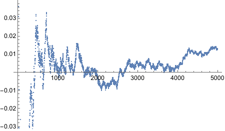
Yes! Looks good! Let’s plot!

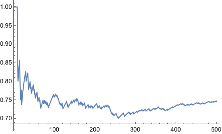
$ListLinePlot [MapIndexed [\frac{Total [biasedtosses [[;; First @ #2]]]}{First @ #2} &, biasedtosses], PlotRange -> All]$

And thus concludes the exercise!

Exercise 4.4

Consider a spinner with a [0,1] scale on its circumference. Suppose that the spinner is slanted or magnetized or bent in some way such that it is biased, and its probability density function is p(x) = 6x(1-x) over the interval x ∈ [0,1].

Adapt the program IntegralOfDensity.R to plot this density function and approximate its integral. Comment your code. Be careful to consider values of x only in the interval [0,1]. Hint: You can omit the first couple of lines regarding meanval and sdval, because those parameter values pertain only to the normal distribution. Then set xlow=0 and xhigh=1, and set dx to some small value.

Derive the exact integral using calculus.

Does this function satisfy equation 4.3?

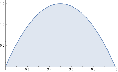
From inspecting the graph, what is the maximal values of p(x)?

Here is the R code from the file:

source("DBDA2E-utilities.R")
# Graph of normal probability density function, with comb of intervals.
meanval = 0.0               # Specify mean of distribution.
sdval = 0.2                 # Specify standard deviation of distribution.
xlow  = meanval - 3.5*sdval # Specify low end of x-axis.
xhigh = meanval + 3.5*sdval # Specify high end of x-axis.
dx = sdval/10               # Specify interval width on x-axis
# Specify comb of points along the x axis:
x = seq( from = xlow , to = xhigh , by = dx )
# Compute y values, i.e., probability density at each value of x:
y = ( 1/(sdval*sqrt(2*pi)) ) * exp( -.5 * ((x-meanval)/sdval)^2 )
# Plot the function. "plot" draws the intervals. "lines" draws the bell curve.
openGraph(width=7,height=5)
plot( x , y , type="h" , lwd=1 , cex.axis=1.5, xlab="x" , ylab="p(x)", cex.lab=1.5, main="Normal Probability Density" , cex.main=1.5 )
lines( x , y , lwd=3 ,  col="skyblue" )
# Approximate the integral as the sum of width * height for each interval.
area = sum( dx * y )
# Display info in the graph.
text( meanval-sdval , .9*max(y) , bquote( paste(mu ," = " ,.(meanval)) ), adj=c(1,.5) , cex=1.5 )
text( meanval-sdval , .75*max(y) , bquote( paste(sigma ," = " ,.(sdval)) ), adj=c(1,.5) , cex=1.5 )
text( meanval+sdval , .9*max(y) , bquote( paste(Delta , "x = " ,.(dx)) ), adj=c(0,.5) , cex=1.5 )
text( meanval+sdval , .75*max(y) ,bquote( sum({},x,{}) *" "* Delta *"x p(x) = "* .(signif(area,3)) ) ,adj=c(0,.5) , cex=1.5 )
# Save the plot to an EPS file.
saveGraph( file = "IntegralOfDensity" , type="eps" )

That’s a lot of code just to display graphs. Disregard those lines, and we are left with a few important lines:

# Specify comb of points along the x axis:
x = seq( from = xlow , to = xhigh , by = dx )

# Compute y values, i.e., probability density at each value of x:
y = ( 1/(sdval*sqrt(2*pi)) ) * exp( -.5 * ((x-meanval)/sdval)^2 )

# Approximate the integral as the sum of width * height for each interval.
area = sum( dx * y )

Fairly straight forward. Initially I thought we are going to use NormalDistribution function, but no. This is just calculating values of “probability density” in a range (0 to 1) with some interval and plots the values. Can we find some excuse to use NormalDistribution?

Anyway, here we go:

$area = Total [y * δ]$

$0.9996$

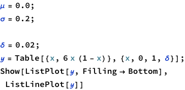
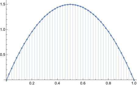
I am curious how the plot looked liked with the original equation.

$\int_{0}^{1} 6 x (1 - x) ⅆ x$

$1$

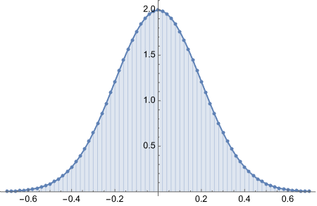
In[296]:=

integrate 6x(1-x) from 0 to 1

$Max [y]$

$1.5$

Thus concludes the exercise.

However, there’s something more we can try. That is to see if we can find more Mathematica-like ways of doing this.
Thinking about it, we are given a probability distribution function 6x(1-x). And all we want is to see how it will behave for different values of the variable x. There is one potential function we can try.

Ah! Look what we got here! Perfect.

$Max [PDF [D, x]]$



6 (1-x) x	0<x<1
0	True

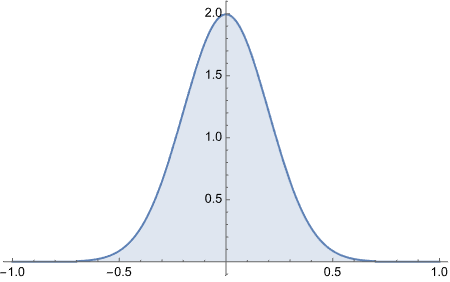
To get area under the curve we do CDF[a] - CDF[b]

$1$

$0.999534741841929$

As you can observe, this approach is much better. Though it may not be as easy to understand what’s really going on under the hood, it is cleaner once you already have understood what’s going on. For example, if we were to start directly with ProbabilityDistribution, we would not know how 6x(1-x) is executed and plotted.

Created with the Wolfram Language